2022 - 2023 H5N1 Bird Flu Modeling and Prediction in the United States

This is an analysis report on the H5N1 Bird Flu outbreak happened since January 2022 in the United States.

Last update: December 20, 2023

Read Report GitHub


University of California, Davis: Weilin Cheng, Hengyuan Liu, Kathy Mo

University of Michigan, Ann Arbor: Sida Tian, Li Yuan

Abstract

Figure 1: Comprehensive Risk Index Map Derived from the XGBoost Model

probability map

This research uniquely focuses on predicting the likelihood of H5N1 outbreaks in the United States at the county level. Unlike previous studies, which either excluded the United States or used outdated data, we utilized diverse statistical techniques and publicly available H5N1-related data from January 2022 to March 2023. Employing logistic regression, regularization methods, cross-validation, and eXtreme Gradient Boosting (XGBoost), our models demonstrated remarkable predictive efficacy. Notably, the XGBoost model, trained with 10-fold cross-validation, outperformed others in terms of ROC-AUC. This research provides valuable epidemiological insights, proposes intervention strategies for H5N1 in the United States, and suggests future research directions.

Introduction

"Egg prices rose to record highs in December. A dozen large Grade A eggs had more than doubled in price during 2022, on average."

— CNBC, Feb. 7 2023

The economic impact of the highly pathogenic avian influenza (HPAI) H5N1 outbreak in the United States has been substantial. Since 2022, the H5N1 virus have been detected across various bird populations, affecting 1,064 counties (Centers for Disease Control and Prevention 2022). Over 58.7 million poultry in 419 counties and approximately 7,105 wild birds in 1,023 counties were infected (Centers for Disease Control and Prevention 2022). In 2022, the H5N1 strain led to an estimated economic loss of \$2.5 to \$3 billion, with around 40 million animal deaths (Farahat et al. 2023). This has brought attention to the United States’ high meat consumption, particularly poultry, which was 115 pounds per capita in 2022 (World Animal Foundation 2023). Additionally, the significant rise in egg prices in 2022 (Iacurci 2023) has disrupted American dietary patterns, indicating broader challenges for the environment and poultry industry.

The primary objective of this study is to develop and evaluate machine learning models that identify areas in the United States at high risk for H5N1 outbreaks, generating predictive insights that can accurately forecast future occurrences in different regions. This approach provides insights to future research on the impact of the H5N1 virus on public health and safety.

Figure 2: Weekly Price of a Dozen of Eggs Since 2019

egg price

Data Processing & Description

To develop a predictive model for identifying counties that might be at risk of H5N1 infection in the future, we need to understand the structure and content of our data. Our approach involves merging five source datasets to create a single, curated dataset that contains all information on H5N1 cases in each county, during a specific month, from January 2022 to March 2023, and a specific outbreak type.
There are 188,580 observations and 10 variables in the curated dataset.

  • fips: Each FIPS code represents a unique county in the United States, so it is a categorical variable with 3,143 unique values, each unique value has 60 entries.
  • state: Abbreviation of each state in the United States, so it is a categorical variable with 51 unique values, each states has its own number of counties.
  • county: The names of counties, independent cities, census areas, and same administrative level regions in the United States, so it is a categorical variable with 3,143 unique values with respect to states, each unique value has 60 entries (note that some sates have some counties with the same name).
  • lat: The latitude of each county.
  • lng: The longitude of each county.
  • month.index: The order of month of avian influenza outbreak from 1 (January 2022) to 15 (March 2023). Each month.index has 12,572 entries. Every month.index has the same number of entries because the cleaned dataset contains all counties’ H5N1 situations regardless of how many cases they have, if there is no cases in a county, then the case number is just 0.
  • type: The type of outbreak in a specific county and month, so it is a categorical variable with 4 unique values, including poultry (47,145 entries), non-poultry (47,145 entries), wild bird (47,145 entries), and captive wild bird (47,145 entries). Every type has the same number of entries because the cleaned dataset contains all counties’ H5N1 situations regardless of how many cases they have, if there is no cases in a county, then the case number is just 0.
  • avg.temp: The average temperature in a specific county and month in Fahrenheit degree (°F).
  • cases: The number of H5N1 cases detected in a specific county and month.
  • binary.case: If the case of a type of outbreak in a specific county and month is 0, then it is marked as uninfected (185,907 entries). Otherwise, it is marked as infected (2,673).

This cleaned dataset will be used to train our classification model to predict which counties might be likely to experience H5N1 infection in the upcoming months.

Source Data:
1. United States Counties Database: https://simplemaps.com/data/us-counties
2. H5N1 Bird Flu Detections across the United States (Backyard and Commercial): https://www.cdc.gov/flu/avianflu/data-map-commercial.html
3. H5N1 Bird Flu Detections across the United States (Wild Birds): https://www.cdc.gov/flu/avianflu/data-map-wild-birds.html
4. Monthly Average Temperature of each County across the United States: https://www.ncei.noaa.gov/access/monitoring/climate-at-a-glance/county/mapping
5. Monthly Average Temperature of each County in Hawaii: https://weatherspark.com/map?id=145043

Visualization

Figure 3: Monthly Distribution of New H5N1 Cases by County in the United States from January 2022 until March 2023

map 1

Figure 4: Monthly Cumulative H5N1 Case Totals by County in the United States from January 2022 until March 2023

map 2

Figure 5: Comprehensive Scatterplot Matrix Depicting
Relationships Among Variables in H5N1 Case Data

scattermatrix

Figure 6: Monthly Distribution of New H5N1 Cases
Visualized in a Bar Chart Format

bar

Models

1. Logistic Regression Model with / without Regularizations

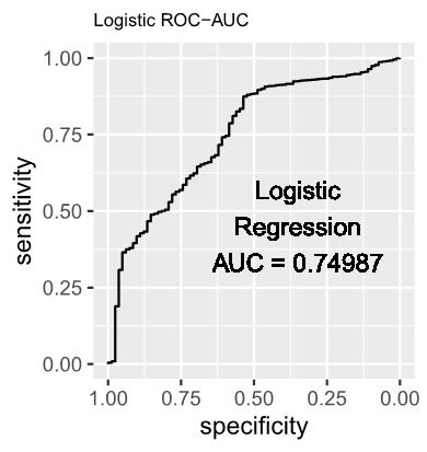
Logistic regression was selected as the baseline model due to its demonstrated effectiveness in accommodating diverse data characteristics. Its appropriateness in the present context lies in its well-established suitability for binary classification tasks, specifically discerning between instances of infected and uninfected status of H5N1 in each county. The mathematical representation of the model is as follows:

\begin{aligned} Y_i = &\beta_0 + \beta_1 \cdot \texttt{lat} + \beta_2 \cdot \texttt{lng} + \beta_3 \cdot \texttt{month.index} + \beta_4 \cdot \texttt{avg.temp} + \beta_5 \cdot \texttt{type(non-poultry)} \\ &+\beta_6 \cdot \texttt{type(poultry)} + \beta_7 \cdot \texttt{type(wild bird)} + \beta_8 \cdot \texttt{lat * lng}. \end{aligned}

The sigmoid transformation below ensures that the predicted probabilities fall within the interval $(0, 1)$, thereby enhancing the model's capability to generate plausible predictions. Serving as a binary classifier, the model is specifically designed to assess the likelihood of H5N1 cases in a county based on the type of outbreak encountered. The application of the sigmoid function contributes to the interpretability and calibration of the model's predictions, aligning them with the probabilistic nature of the logistic regression framework.

\begin{aligned} &\Pr(Y_i=\texttt{infected} | X_i) = p(X_i) = \frac{e^{\beta_0 + \beta_1 \cdot \texttt{lat} + ... + \beta_8 \cdot \texttt{lat * lng}}}{1 + e^{\beta_0 + \beta_1 \cdot \texttt{lat} + ... + \beta_8 \cdot \texttt{lat * lng}}}\\ &\Pr(Y_i=\texttt{uninfected} | X_i) = 1 - p(X_i) = 1 - \left(\frac{e^{\beta_0 + \beta_1 \cdot \texttt{lat} + ... + \beta_8 \cdot \texttt{lat * lng}}}{1 + e^{\beta_0 + \beta_1 \cdot \texttt{lat} + ... + \beta_8 \cdot \texttt{lat * lng}}}\right). \end{aligned}

1.1 The estimated log-odds of the Logistic Regression Model is as follows:

\begin{aligned} \hat{Y}_i = &18.215 - 0.284 \cdot \texttt{lat} + 0.08 \cdot \texttt{lng} - 0.057 \cdot \texttt{month.index} - 0.004 \cdot \texttt{avg.temp} - 0.203 \cdot \texttt{type(non-poultry)} \\ &-0.055 \cdot \texttt{type(poultry)} - 1.997 \cdot \texttt{type(wild bird)} - 0.002 \cdot \texttt{lat * lng}. \end{aligned}

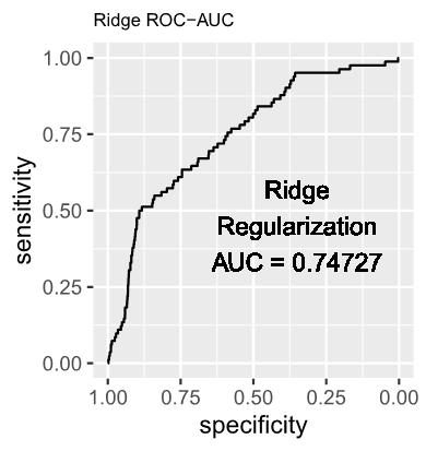
1.2 The estimated log-odds of the Logistic Regression Model with Ridge (L2) Regularization is as follows:

\begin{aligned} \hat{Y}_i = &9.092 - 0.085 \cdot \texttt{lat} + 0.006 \cdot \texttt{lng} - 0.048 \cdot \texttt{month.index} - 0.001 \cdot \texttt{avg.temp} + 0.043 \cdot \texttt{type(non-poultry)} \\ &+0.168 \cdot \texttt{type(poultry)} - 1.693 \cdot \texttt{type(wild bird)} - 5.818\times 10^{-5} \cdot \texttt{lat * lng}. \end{aligned}

1.3 The estimated log-odds of the Logistic Regression Model with Lasso (L1) Regularization is as follows:

\begin{aligned} \hat{Y}_i = &17.243 - 0.262 \cdot \texttt{lat} + 0.072 \cdot \texttt{lng} - 0.056 \cdot \texttt{month.index} - 0.004 \cdot \texttt{avg.temp} - 0.197 \cdot \texttt{type(non-poultry)} \\ &-0.049 \cdot \texttt{type(poultry)} - 1.99 \cdot \texttt{type(wild bird)} - 0.002 \cdot \texttt{lat * lng}. \end{aligned}

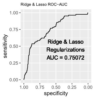
1.4 The estimated log-odds of the Logistic Regression Model with Ridge (L2) and Lasso (L1) Regularizations is as follows:

\begin{aligned} \hat{Y}_i = &17.278 - 0.263 \cdot \texttt{lat} + 0.072 \cdot \texttt{lng} - 0.056 \cdot \texttt{month.index} - 0.004 \cdot \texttt{avg.temp} - 0.197 \cdot \texttt{type(non-poultry)} \\ &-0.05 \cdot \texttt{type(poultry)} - 1.991 \cdot \texttt{type(wild bird)} - 0.002 \cdot \texttt{lat * lng}. \end{aligned}

2. eXtreme Gradient Boosting (XGBoost) Model

In contemporary times, XGBoost has emerged as a robust ensemble learning technique, garnering widespread acclaim for its exceptional predictive prowess. The algorithm methodically assembles a set of weak learners, typically manifested as decision trees, and amalgamates their predictions to bolster accuracy and exhibit strong generalization performance on unseen data.

The XGBoost model was trained utilizing the exact tree method, and its performance was systematically monitored through the negative log-likelihood loss at each iteration of the training process. In order to ensure both performance and robustness, a 10-fold cross-validation strategy was implemented at each training round, and certain hyperparameters were systematically adjusted and applied as delineated below:

  • The learning rate ($\eta$) was designated as 0.02, serving as the step size shrinkage to mitigate overfitting during the training process.
  • The subsample ratio was established at 0.75, indicating that the XGBoost algorithm would stochastically select 75% of the training data for each tree's growth.
  • The column subsample ratio for each tree was configured to 0.8, signifying that the XGBoost algorithm would randomly consider 80% of predictors when developing a new tree.
  • The maximum depth of the trees was restricted to 10.
  • The number of training rounds was predetermined to be 700.

Figure 7: Training and Validation Losses of XGBoost Model over 700 Rounds of Training

xgbloss

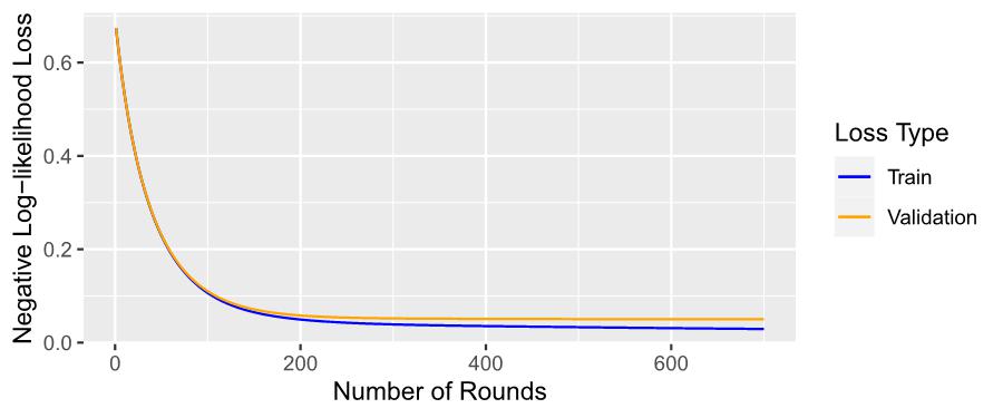
Figure 7 illustrates the progression of training and validation losses across 700 rounds. The training loss, depicted by the blue line, exhibits a consistent and gradual decrease over the course of the training iterations. Similarly, the validation loss, represented by the orange line, also demonstrates a continuous and steady decline.

Figure 8: Feature Importance Plot for XGBoost Model

xgbimportance

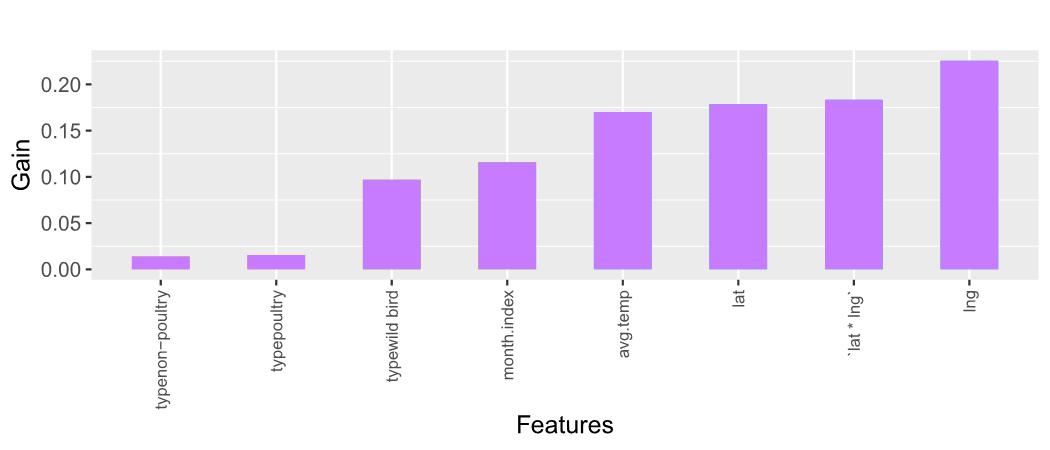
Figure 8 depicts the Gain scores associated with the predictors employed in the XGBoost model. A taller bar, indicative of a higher Gain score, signifies greater importance of the corresponding predictor. Remarkably, pivotal predictors such as lng (longitude), lat * lng (interaction between latitude and longitude), and lat (latitude) have emerged as noteworthy contributors to the predictive efficacy of the model.

Model Selection and Evaluation

Given the test accuracy of these models are all 99% and the fact that the dependent variable binary.cases has imbalanced classes, the test ROC-AUC is the preferred metric here.

Figure 9: Receiver Operating Characteristic (ROC) Curves for Model Discrimination

logistic ROC-AUC
l2 ROC-AUC
l1 ROC-AUC
l2l1 ROC-AUC
all ROC-AUC
xgb ROC-AUC

In Figure 9, the XGBoost model demonstrates exceptional efficacy, as evidenced by a remarkable test ROC-AUC score of 0.87928. This superiority is discernible when juxtaposed against traditional models such as Logistic Regression, Logistic Regression with Lasso Regularization, Logistic Regression with Ridge Regularization, and their amalgamated approach

Figure 10 provides an in-depth examination through a series of risk index maps, which divide the United States into four distinct regions: West, South, Midwest, and Northeast. Risk index is the cumulative predicted probabilities, generated by the XGBoost Model, for all four potential H5N1 outbreak types (poultry, non-poultry, wild bird, and captive wild bird) across all counties in March 2023. The presence of documented H5N1 cases is represented by green dots within these regions, and the size of each green dot is scaled to reflect its contextual significance within the respective region, aiming to amplify visual impact. Additionally, blue triangles within each region pinpoint counties with reported cases and a risk index exceeding 0.25.

Figure 10: Risk Index Map by Regions Derived from the XGBoost Model

regional_risk

It is evident that West and South regions experienced the fewest outbreaks in March 2023 among the four delineated regions. Specifically, within the West region, six counties are marked by blue triangles - three in California, two in Colorado, and one in Oregon. The South region exhibits a total of two counties with blue triangles, all located in Florida. In the Midwest region, there is a solitary county, situated in Minnesota, marked by a blue triangle. However, it is noteworthy that the county highlighted is not necessarily the one with the highest incidence of H5N1 cases, because the size of the green dot is not the largest in the region. The Northeast region endured the most severe H5N1 outbreak in March 2023 among the four regions. Four counties are identified by blue triangles, with particular emphasis on the county in Pennsylvania, which recorded the highest number of H5N1 outbreak cases. Noteworthy is the commendable performance of the XGBoost model, which accurately identifies the Northeast region as particularly risky.

Conclusion & Suggestions

In this study, logistic regression, model regularization techniques, 10-fold cross validation, and eXtreme Gradient Boosting (XGBoost) have been methodically utilized to predict the probability of H5N1 outbreaks in the United States. The study's results demonstrate a notably high ROC-AUC score of 0.87928 for the XGBoost model, underscoring its effectiveness in forecasting future H5N1 cases. This model has accurately pinpointed counties in the United States, particularly in the Northeast region, with an elevated risk of H5N1 outbreaks in March 2023, which corresponds closely with the actual outbreak patterns observed. Within this context, geographic factors emerged as the most critical features in the XGBoost model. Additionally, the variable of temperature was identified as a subsequent pivotal feature, aiding in the guideline of H5N1 risk control across various U.S. counties.

However, the study acknowledges certain limitations in its methodology. The predictive models predominantly considered variables such as temperature, types of outbreaks, time, and population density. Critical factors like existing control zones, wild waterfowl migration patterns, agricultural practices, off-site daily mortality disposal methods, and wild bird access to feed (Green et al. 2023), which could significantly influence H5N1 spread, were not incorporated.

To augment the robustness and precision of our models, future studies should incorporate more comprehensive datasets, including factors like bird migration, human travel patterns, and agricultural data. Exploring advanced machine learning techniques, such as Convolutional Neural Networks (CNNs) and time series analysis, is recommended to elucidate the intricate interactions among these variables. The efficacy of CNNs in related fields is exemplified in the work of Scarafoni et al. (2019), who adeptly applied deep CNN models to predict the host tropism of the Influenza A virus based on protein sequences, thereby demonstrating the potential of this method in virological studies. Furthermore, integrating time series techniques with tree models such as Random Forest and XGBoost, as demonstrated by Kane et al. (2014) in their analysis of H5N1 outbreak predictions in Egypt, could yield low mean square error (MSE) in both retrospective (MSE = 6.3195) and prospective (MSE = 24.8101) contexts. Additionally, the application of Long Short-Term Memory (LSTM) networks, as shown in the study "Prediction of COVID-19 using long short-term memory by integrating principal component analysis and clustering techniques," (Ilu, Rajesh, and Mohammed 2022) underscores the viability of LSTM in H5N1 research. This study reported both sensitivity and specificity rates of 98% for the LSTM model, indicating its commendable performance in disease forecasting.

Our study identifies geographical location and temperature as key predictors in distinguishing between infected and uninfected cases in our model. "Technical Report: Highly Pathogenic Avian Influenza A(H5N1) Viruses" from Disease Control and Prevention highlights the current low public health risk posed by A(H5N1) viruses. However, the widespread geographic distribution of infected birds and poultry, along with the potential for human and mammalian exposures, increases the likelihood of viral evolution or reassortment events, potentially altering the risk assessment. This underscores the connection between H5N1 infection and geographic factors, corroborating our model’s emphasis on these variables. Additionally, the study "Avian Influenza Virus (H5N1); Effects of Physico-Chemical Factors on Its Survival" conducted by Shahid et al. (2009) reveals a significant relationship between Avian Influenza Virus H5N1 infection and temperature, demonstrating that the virus maintains infectivity at 4 degrees Celsius (39.2 Fahrenheit) for over 100 days, although hemagglutinin (HA) activity diminishes. In contrast, the virus loses its infectivity after 24 hours at room temperature 28 degrees Celsius (82.4 Fahrenheit).

Future research, building on our study's insights, should delve deeper into the intricate relationships among spatial, time, and temperature factors. Emphasizing the geographical location and temperature as pivotal predictors, researchers could explore the spatial dynamics of H5N1 outbreaks with a finer resolution, considering not only county-level data but also incorporating more granular information to capture localized patterns. Additionally, investigating the interactions among spatial, time, and temperature variables can provide a more nuanced understanding of the dynamics influencing the spread of the virus. Integrating advanced spatial analysis techniques, such as Geographic Information System (GIS) mapping, can help uncover spatial patterns that may not be immediately apparent, contributing to a more comprehensive predictive model.

In addition to research directions, comprehensive datasets would enable a more holistic analysis of the multifaceted aspects influencing H5N1 transmission. Collaborative efforts among researchers, governmental agencies, and international organizations can facilitate the sharing of standardized data, fostering a collective approach to understanding and combating the potential threats posed by H5N1 outbreaks.

By focusing on these research directions, scientists can contribute to the development of more robust and accurate predictive models, ultimately aiding in proactive measures for H5N1 risk management and control.